Demand and Supply
Let’s set the one and only ground rule for this article i.e. Ceteris paribus
Ceteris paribus : A Latin phrase that generally means “all other things being equal.”
For the purpose of our article we will use this to define the state of the market or the products. That means no new advancement of technologies, new features in product or any better quality products has been introduce in the market to change the state of demand and supply of a product or service in a market. For example, the value of iPhone 11 will automatically drop down when iPhone 12 is launched in the market. This scenario will never occur in our assumption.
First let’s have a look at a general demand and supply curve.

Demand Curve
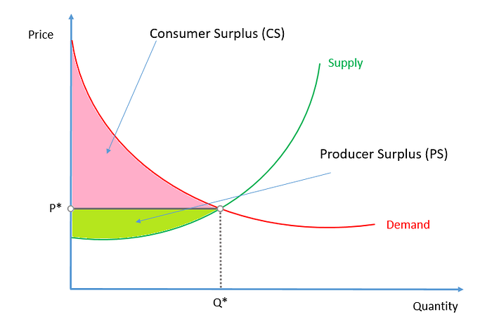
The demand curve gives us the quantity of a product that a consumer is ready to purchase at a given price. In Basic economics we only consider two factors which is the price and quantity, all other factors are considered as constant for ease of understanding.
In the above plot we can see lesser the price more is the quantity in demand.
Supply Curve
Since now we understand the demand curve, a supply curve is very easy to understand. It is the relationship between various prices and the quantity offered by producers at each price point.
The equilibrium point i.e. P* and Q* are the points where the supply of a product exactly meets the demand in the market.

Consumer Surplus
A consumer surplus is the difference between the equilibrium price and the highest price people are willing to pay for a product.
Producer Surplus
Its the difference between the selling price of a product and what the producer might have agreed to sell the product for.
The Sum of both consumer surplus and producer surplus gives us the Welfare. This is the overall economic welfare of the society we can calculate just by looking at the demand and supply curve.
Welfare = Consumer surplus + Producer Surplus
Costs of a produce
Before we understand markets lets understand the different costs that effect the produce.
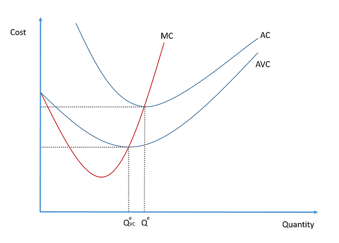
- Marginal Cost: Its the cost that is incurred to produce one extra unit of the product.
- Average Variable Cost: Its the variable cost/ total number of units produce.
- Average Total Cost : Total cost of the firm/total output.
The general graph for the above three costs in the short run helps us determine the quantity of a product which should be produced so that we can maximize the profits.

The point where the marginal cost is equal to the Average cost (Average Total Cost) gives us the quantity (Qe)which can be produced in minimum cost per unit. Any production above that point will result in increasing the cost of production per unit.
The MC Curve
The general nature of the MC curve is that the MC value will fall initially when the production increase and after a point the MC values will start to increase. This happens because as the production increases we need to put in more and more assets in the shop floor to produce more number of products, which increases our marginal cost.
Marginal cost is an important factor in understanding different markets as it helps us determine the profits as well as optimize the profits by optimizing the production.
Somewhere in a separate section we will also go over different type of markets in detail which are broadly divided into
1. Perfect Competition Market
2. Monopolistic Competition Market
3. Oligopoly Market
4. Monopoly Market
These market categorization occurs based on the extent of product differentiation offered by the competition in the market and the total numbers of firms present in the market.
